Intro / Motivation / Why
The code, functions and algorithms we write are not all the same. One very important aspect in which they differ is the complexity and efficiency. In order to produce quality solutions and improve existing ones, it would be great if there was a way to measure this somehow. Is there a way to measure this difference mathematically? Yes! We do this using the "Big O Notation"
What is "Big O Notation"?
Now that we have the why out of the way, let's look at the "what". Skipping the, usually, confusing wikipedia definition, let's try something simpler...
Big O notation is a mathematical description of algorithmic complexity relative to time and space i.e. a description of how much time or resources an algorithm will consume with increasing input size.
How Does Big O Break Down Complexity?
Big O notation breaks complexity down by the amount of time and space an algorithm uses relative to the input. An algorithm then falls into one of the following notations:
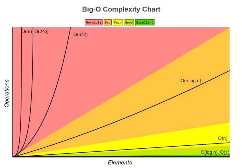
So our algorithms can be have one of the following complexities:
1. O(1)
Time or space is independent of input size e.g.:
- input 2 - time 1
- input 4 - time 1
- input 8 - time 1
2. O(log n)
Time or space increases based on every doubling of input size e.g.:
- input 2 - time 2,
- input 4 - time 3,
- input 8 - time 4
3. O(n)
Time or space increase is directly tied the input size e.g.:
- input 2 - time 2,
- input 4 - time 4,
- input 8 - time 8
4. O(n log n)
Time or space doubles as input size increases e.g.:
- input 2 - time 4,
- input 4 - time 8,
- input 8 - time 16
5. O(n^2)
Time or space increases quadratically as input size increases e.g.:
- input 2 - time 4,
- input 4 - time 16,
- input 8 - time 64
6. O(2^n)
Time or space increases exponentially as input size increases e.g.:
- input 2 - time 4,
- input 4 - time 16,
- input 8 - time 256
7. O(n!)
Time or space increases factorially as input size increases e.g.:
- input 2 - time 2,
- input 4 - time 24,
- input 8 - time 40320
As we can see, the different complexities can have dramatic impact.
NOTE: Algorithms are not limited to one of the above but can have multiple complexities depending on the input. This means they can have a best case, an average and a worst case scenario.
Show Me The Code!
First Element
Let's take the following example (Javascript) ...
function getFirstElement(array) {
  return array[0];
}
This is an O(1) complexity because the time required for the execution is independent of the input array length. Unfortunately, only a few algorithms can be this fast.
Bubble Sort
Let's take another example (Javascript) ...
function bubbleSort(array) {
  while (true) {
    let swapped = false;
    for (let i = 0; i < array.length; i++) {
      // if next element is bigger swap
      // the current with the next
      const nextElement = array[i+1]
      if(nextElement != undefined && array[i] > nextElement) {
        const temp = array[i]
        array[i] = nextElement;
        array[i+1] = temp;
        swapped = true;
      }
    }

    // finish if there was no swap after
    // a full traversal over all elements
    if (! swapped) {
      break;
    }
  }

  return array;
}
This bubble sort algorithm iterates over an array over and over again comparing the current and next element in the array. If the current is bigger than the next, it swaps the two. It does this until it doesn't detect a swap after a full input array iteration.
Let's visualize it for better understanding ...
First full traversal of the input array:
[6, 4, 5, 3, 2, 1] → [4, 6, 5, 3, 2, 1] - swap
[4, 6, 5, 3, 2, 1] → [4, 5, 6, 3, 2, 1] - swap
[4, 5, 6, 3, 2, 1] → [4, 5, 3, 6, 2, 1] - swap
[4, 5, 3, 6, 2, 1] → [4, 5, 3, 2, 6, 1] - swap
[4, 5, 3, 2, 6, 1] → [4, 5, 3, 2, 1, 6] - swap
swapped = true
Second full traversal of the input array:
[4, 5, 3, 2, 1, 6] → [4, 5, 3, 2, 1, 6]
[4, 5, 3, 2, 1, 6] → [4, 3, 5, 2, 1, 6] - swap
[4, 3, 5, 2, 1, 6] → [4, 3, 2, 5, 1, 6] - swap
[4, 3, 2, 5, 1, 6] → [4, 3, 2, 1, 5, 6] - swap
[4, 3, 2, 1, 5, 6] → [4, 3, 2, 1, 5, 6]
swapped = true
...
This goes on until we have a full traversal without any swaps ...
[1, 2, 3, 4, 5, 6] → [1, 2, 3, 4, 5, 6]
[1, 2, 3, 4, 5, 6] → [1, 2, 3, 4, 5, 6]
[1, 2, 3, 4, 5, 6] → [1, 2, 3, 4, 5, 6]
[1, 2, 3, 4, 5, 6] → [1, 2, 3, 4, 5, 6]
[1, 2, 3, 4, 5, 6] → [1, 2, 3, 4, 5, 6]
swapped = false
So what is the complexity of this? For the sake of brevity we'll only determine the worst case scenario.
If we use the input [8, 7, 6, 5, 4, 3, 2, 1] and build in an iterations counter we will see that for an input of 8 we the algorithm uses 64 iterations.
If we check the previously mentioned big O notations we will see that O(n^2) gives us a time complexity of 64 for an input of 8.
Is Big O Always Decisive?
You know how our physics rules don't work on the quantum scale? Well Big O is kinda similar i.e. for small inputs one algorithm can seemingly be much faster than another but do we really care if something took 1ms or 5ms? We might, in rare cases but what really matters for the vast majority of us is the difference between e.g. 500ms and 4s. So Big O is much more useful for the bigger scale and larger inputs rather then small inputs where some algorithms can be faster than others but then break down and take much more time for larger inputs.
Conclusion
The Big O notation is a good tool that every software engineer should be aware of. It helps us describe algorithm complexity and as such it can be beneficial to keep it in mind when writing and optimizing our solutions.